Forecasting Global Food Production Emissions: A Time Series Case Study

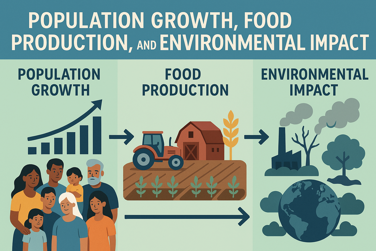
Understanding the environmental impact of global food production is crucial, especially with a growing world population. This project dives into historical data to analyze trends and build forecasting models for food production quantities and their associated emissions. The goal was to leverage time series analysis techniques to provide insights that could inform sustainability efforts.

The Challenge: Integrating Diverse Datasets

The project started with three distinct datasets spanning several decades:

1. FAO Food Production (1961-2013): Yearly data on food produced for human nutrition vs. animal feed, per country.
2. World Population (1960-2018): Population data for each country from the World Bank.
3. Food Emissions: Environmental impact (water, soil, carbon footprint) data for 43 common food products.

Integrating these datasets presented several challenges: different time ranges, units of measurement (tonnes vs. kg), inconsistent category naming (food items), missing data, and the inherent non-stationarity often found in time series data exhibiting trends.

Building the Data Pipeline: Cleaning, Transformation, and Feature Engineering

A significant portion of the project involved creating a robust data pipeline using Python and pandas to prepare the data for analysis and modeling.

Data Acquisition and Initial Cleaning

• Loading: Data was loaded from various sources.
• Filtering: Initial cleaning involved filtering the FAO dataset to focus only on “Food” production, removing “Feed” data.
• Unit Conversion: Production quantities were converted from ‘1000 tonnes’ to kilograms to align with the emissions data. The original ‘Unit’ column was then dropped.
• Handling Missing Data: Missing values were assessed per column and row.
  • Rows with over 80% missing data (e.g., Montenegro) were strategically removed.
  • Historical missing data blocks (often at the start of a country’s record-keeping) were noted but retained, as time series models can handle leading NaNs. Imputation wasn’t deemed appropriate for these large initial gaps.
• Outlier Consideration: Standard outlier detection methods (like IQR) flagged some data points in the emissions and population datasets. However, after review, these were deemed contextually valid (e.g., high emissions for meat products used as animal feed, large populations for countries like China/India). Removing them could distort the analysis, so they were kept.
• Dimensionality Reduction: The emissions dataset was simplified by removing metrics based on kcal and protein, focusing on per-kilogram emissions for direct correlation with production quantities.

Data Transformation and Merging

• Reshaping: The FAO production and World Bank population datasets, originally in a wide format (years as columns), were transformed into a long format using pandas.melt(), making them suitable for time series analysis.
• Standardization: Column names like ‘Area’ and ‘Country Name’ were standardized to ‘Country’ across datasets to facilitate merging.
• Category Mapping: A crucial step was mapping the different names used for similar food items across the FAO and Emissions datasets (e.g., “Wheat & Rye (Bread)” to “Wheat and products”). This required creating a custom mapping dictionary.
• Joining: The cleaned and transformed datasets were merged sequentially based on common keys (‘Country’, ‘Year’, ‘Item’) into a final comprehensive DataFrame.

Feature Engineering

• Total Emissions: A key engineered feature, ‘Emissions Production’, was calculated by multiplying the food ‘Quantity’ (in kg) by the corresponding ‘Total_emissions’ factor (emissions per kg) for each food item, country, and year.

Time Series Analysis and Modeling

With the cleaned and merged dataset, the focus shifted to time series analysis and forecasting.

Exploring Trends and Stationarity

• Visualization: Initial plots of global production quantities and calculated emissions over the years revealed clear upward trends, indicating non-stationarity.
• ADF Testing: The Augmented Dickey-Fuller (ADF) test confirmed the non-stationarity of the raw time series (p-value >> 0.05).
• Differencing: To achieve stationarity, first-order differencing was applied to the time series data (.diff()). The ADF test on the differenced data showed stationarity (p-value << 0.05).
• Decomposition: The differenced time series was decomposed into trend, seasonality (though minimal given yearly data), and residuals using statsmodels.tsa.seasonal.seasonal_decompose. Residual analysis (mean close to zero, ACF/PACF plots) helped validate the differencing approach.

Establishing Baselines and Advanced Models

Forecasting models were developed for the aggregated global ‘Quantity’ and ‘Emissions Production’ time series:

• Baseline: A NaiveForecaster (predicting the last observed value forward) was used as a benchmark.
• ARIMA: AutoARIMA from pmdarima (and sktime) was used to automatically find the optimal (p, d, q) orders for separate forecasts of ‘Quantity’ and ‘Emissions Production’. Stationarity was addressed via differencing (d=1 or d=2 found by AutoARIMA).
• VAR (Vector Autoregression): A VAR model from statsmodels was implemented to model ‘Quantity’ and ‘Emissions Production’ simultaneously, capturing potential interdependencies between food production and its emissions. Stationarity was again addressed via differencing before model fitting.
• XGBoost (Experiment): An XGBoost regressor was briefly tested using only ‘Year’ as a feature. It significantly underperformed, likely due to the limited features and the relatively small number of data points (years) for a complex machine learning model.

Evaluating Forecasts

Models were evaluated against a held-out test set using Mean Absolute Percentage Error (MAPE).

• Naive MAPE: ~16.0% (Quantity), ~13.2% (Emissions)
• ARIMA MAPE: ~4.6% (Quantity), ~1.9% (Emissions)
• VAR MAPE: ~3.5% (Quantity), ~3.2% (Emissions)

Both ARIMA and VAR models significantly outperformed the naive baseline. VAR showed slightly better performance for Quantity, while ARIMA was better for Emissions, suggesting a trade-off depending on the primary target variable. Visual inspection confirmed forecasts generally followed the trends observed in the test data.

Key Outcomes and Learnings

• Successfully constructed an end-to-end data pipeline to ingest, clean, transform, and merge data from multiple disparate sources.
• Applied appropriate time series analysis techniques, including stationarity testing (ADF), differencing, and decomposition.
• Developed and compared multiple forecasting models (Naive, ARIMA, VAR), demonstrating a significant improvement over baseline methods.
• Gained insights into the historical trends linking population growth, food production, and emissions on a global scale.

Conclusion

This project successfully demonstrated the process of tackling a complex time series forecasting problem using real-world data. While the global-level ARIMA and VAR models provide valuable high-level forecasts, future work could involve building more granular models (per-country or per-food-item) or exploring machine learning approaches with richer feature sets if more relevant data were available. The analysis provides a foundation for understanding long-term trends in food system sustainability.